Build a Flow
This guide walks through building a flow for ingesting plate reader absorbance data captured at two timepoints and computing the difference between the two values.
Flows are programs represented as directed graphs comprised of user-editable nodes. For more information on flows and nodes, check out the Ganymede Concepts page.
Step 0: Download sample plate reader file
Click on this link to download the plate reader file used for this tutorial.
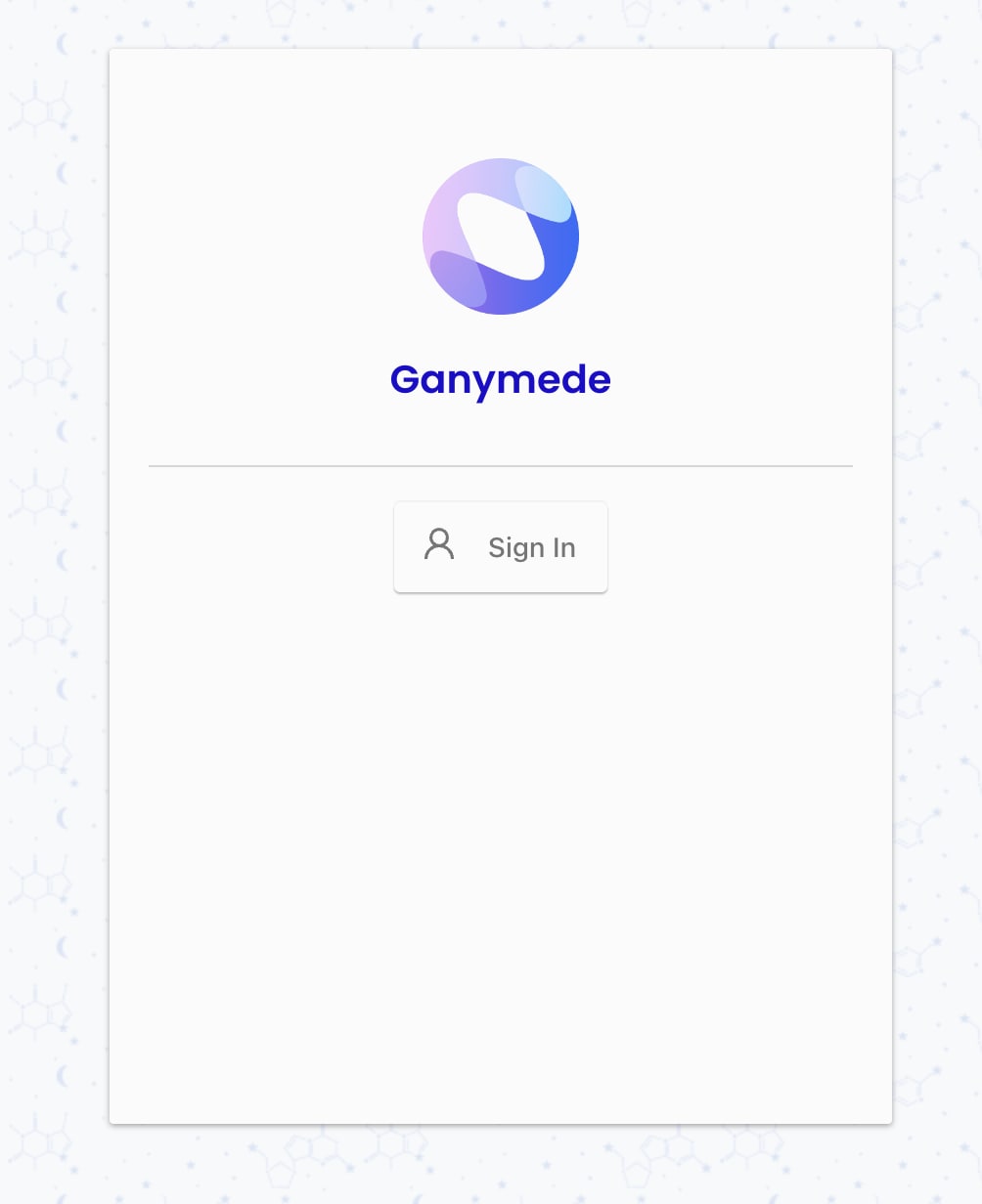
Step 1: Sign into Ganymede
The
button should be available once authentication is configured for your tenant, which is generally going to be a web address accessible via any web browser with the URL https://<your_tenant>.ganymede.bio.You may need to enable pop-ups for Ganymede or disable any ad-blocking software for the ganymede.bio domain.
Step 2: Select the Flow Editor page
Click on the
button in the sidebar.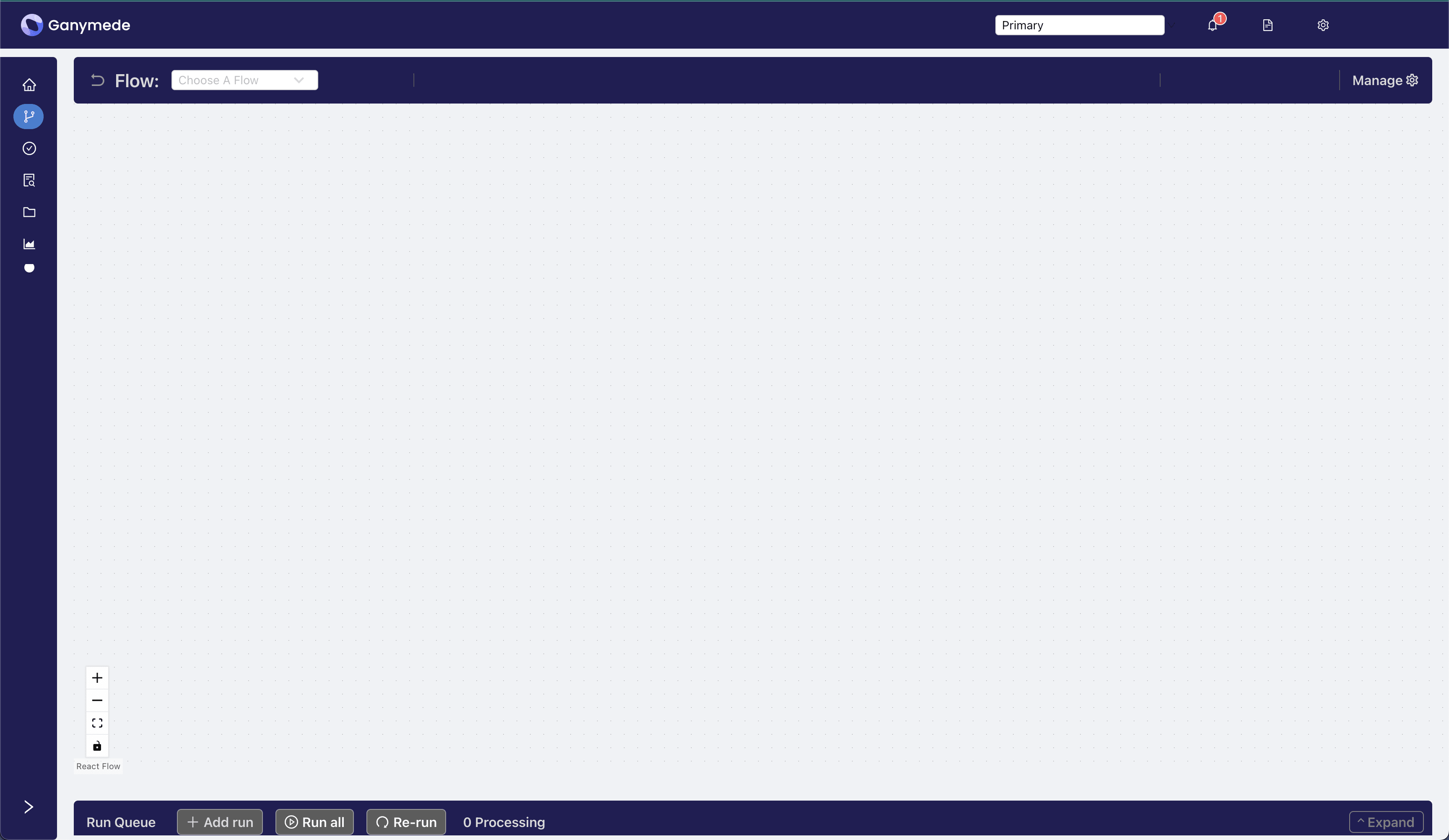
Step 3: Create a new flow
Click on the
button in the upper right-hand corner of the header bar and select from the right sidebar.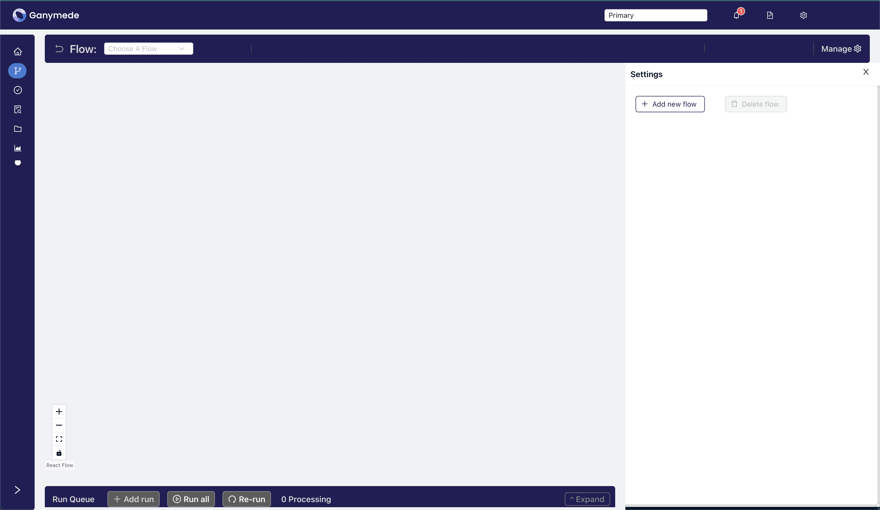
This exposes a modal for adding a new flow. Name the flow "Quickstart_Absorbance_Change" as shown below, add a description, and then hit the "Create Flow" button.
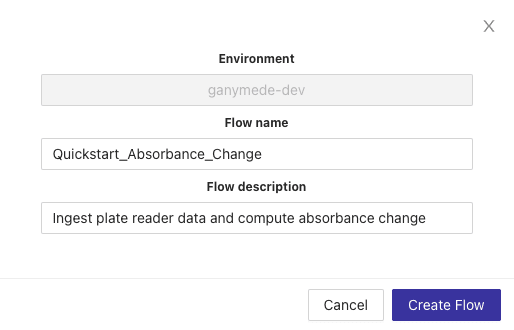
After a few seconds, your flow will be created and you'll be redirected to a blank flow editor page where you can edit your new flow.
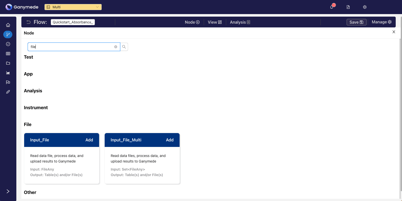
Step 4: Add nodes to ingest and process data
Click on the
button in the header bar and search for the term "input" to filter for the relevant node. Click the button to add it to your flow.The Input File Multi node can be used to ingest multiple files on a single node. For this quickstart, we will use the Input File node to ingest a single file.
Click on the downward-pointing carat in the corner of the
node to expand it and edit its attributes. Change the file_pattern node attribute from "file_pattern" to "*.xlsx" so that only files with.xlsx as an extension will be processed by this node (other file types, such as .csv will be blocked).
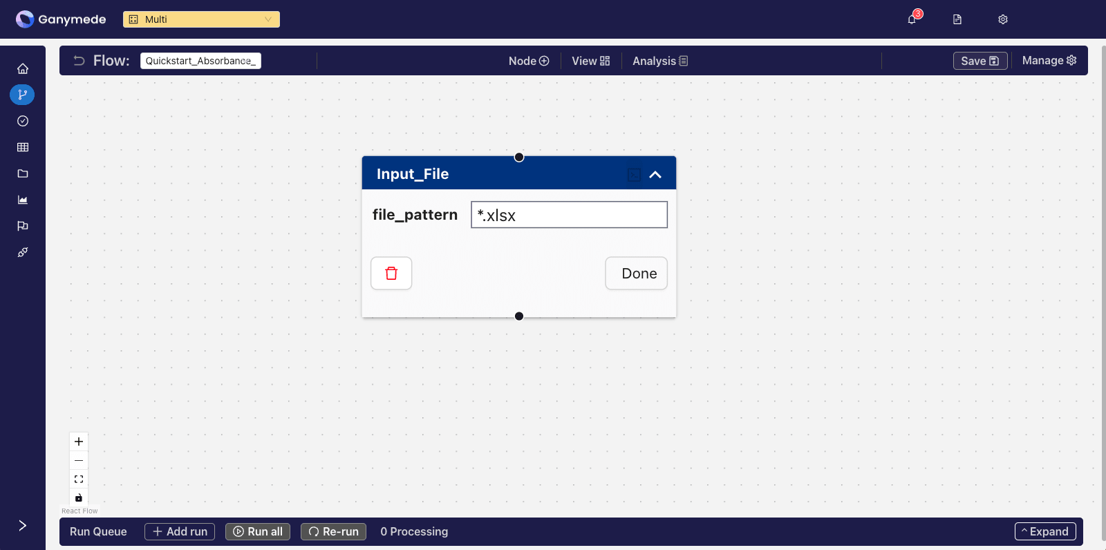
Extension validation can be removed by leaving the file validation node attribute blank.
Click
in the header to save this change.A message will pop up in the upper right when the Save is complete. You can also click the button in the upper right corner to view the Notifications page where you can track the progress of a Save.
Now you have a one-node flow that is capable of ingesting Excel files. Let's add a second node to process this incoming raw data into some useful output.
Click on the
button in the header bar again, and search for the term "Python". This time, we want to add a node to our flow. Click the button to add it to your flow.Upon doing so, the
window should look as follows: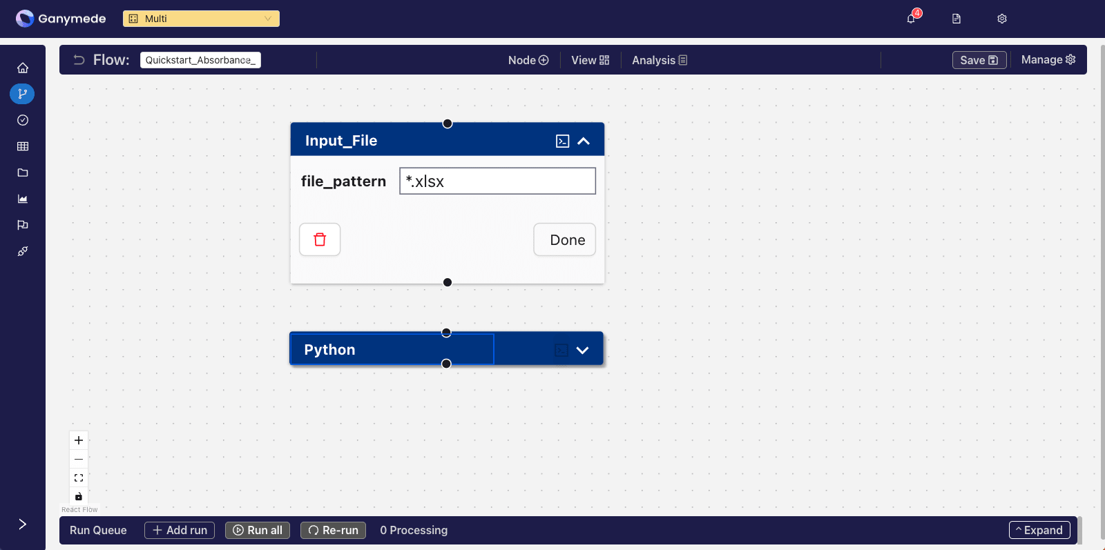
Of course, we want data processing to flow from the
node to the node. To effectuate this, click on the node's bottom attachment point and drag the connection to the top of the node. Then click .Step 5: Modify the Input File node to store results in a table
Expand the
node by clicking on the downward-pointing carat in the corner of the node. Click on the command prompt icon in the upper-right-hand corner of the node to edit the Python code associated with node.We will output the contents of the plate reader spreadsheet into a cloud database table called Quickstart_Absorbance_Change_data by modifying the contents of the User-Defined Function cell as shown below. Simply copy and paste all the code below into the notebook cell.
from typing import Dict
from ganymede_sdk.io import NodeReturn
import pandas as pd


def execute(file_data: Dict[str, bytes], ganymede_context=None) -> NodeReturn:
    """
    Processes file data for saving in cloud storage

    Parameters
    ----------
    file_data : Dict[str, bytes]
        Bytes object to process, indexed by filename
    ganymede_context : GanymedeContext
        Ganymede context variable, which stores flow run metadata

    Returns
    -------
    NodeReturn
        Table(s) and File(s) to store in Ganymede.  To write to the table referenced on the node,
        return a DataFrame in the "results" key of the tables_to_upload dictionary.  For more info,
        type '?NodeReturn' into a cell in the editor notebook.
    """

    excel_file = list(file_data.values()).pop()
    df_excel_file = pd.read_excel(excel_file)

    return NodeReturn(
        tables_to_upload={'Quickstart_Absorbance_Change_data': df_excel_file},
    )
Non-tabular data can be stored by returning a dictionary of files to upload in the files_to_upload key of the NodeReturn object.
Run the User-Defined Function cell by selecting the cell and then clicking on the
button in the header, which runs the selected cell. In the "Testing" section below, you can test out uploading our original plate reader excel file and passing it into the User-Defined Function. This is a great way to debug your code before deploying the flow.Save and deploy changes made to the Python node by clicking on the button in the toolbar, or by pressing Cmd+S (Mac) or Ctrl+S (Windows/Linux).
Below the User-Defined Function cell in the notebook, you'll find the Testing Section. Here, you can upload a test input file and test the processing performed by the User-Defined Function interactively. This is a great way to debug your code before deploying the flow.
Step 6: Modify the Python node to calculate absorbance difference
Right now the
node is in its default state, so let's edit it to make it do some processing specific to our Plate Reader data. To do so, open up the backing notebook for by clicking on the command prompt icon in the upper-right-hand corner of the node.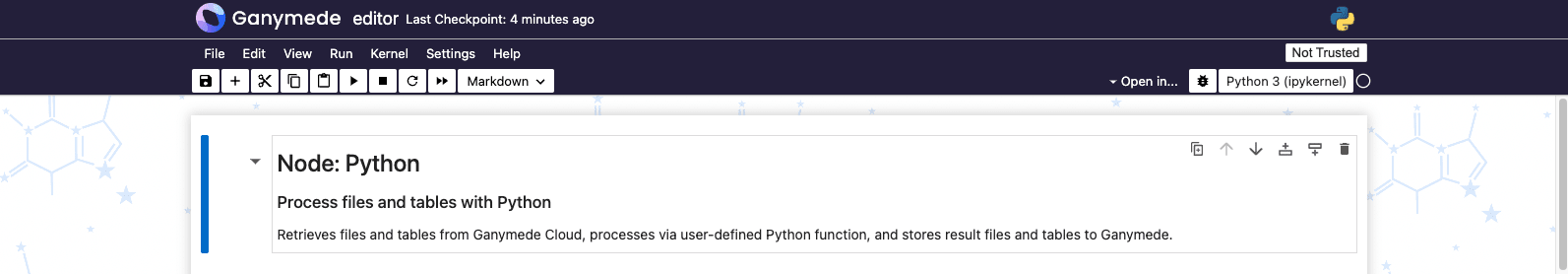
Edit the query_sql string to query for the output of the
query_sql = """
  SELECT * FROM Quickstart_Absorbance_Change_data
"""
Since the plate reader file has been ingested in the
node, we now can query the results of that node using a SQL query on the tableQuickstart_Absorbance_Change_data. The query above simply selects all the data from this table.
Run this notebook cell by clicking on the
button in the header.Next, modify the User-Defined Function cell to calculate the absorbance difference as follows, and run the cell:
import pandas as pd
from ganymede_sdk.io import NodeReturn
from typing import Union, Dict, List

def execute(
    df_sql_result: Union[pd.DataFrame, List[pd.DataFrame]], ganymede_context=None
) -> Union[pd.DataFrame, Dict[str, pd.DataFrame]]:

    # remove fields that do not contain well measurements
    df_out = df_sql_result[~df_sql_result['field'].isin(['Cycle Nr.', 'Time [s]', 'Temp. [°C]'])].copy()

    # calculate absorbance difference
    df_out['run_diff'] = df_out['run2'] - df_out['run1']

    return df_out
This takes the difference between the two columns run1 and run2, and stores the result in a new column called run_diff.
Near the bottom of the notebook you'll find the Testing Section. As with the Input_File node, you can test out the SQL query and the User-Defined Function interactively.
After saving the flow, close the editor notebook associated with the Python node to return to the
view.Step 7: Run the flow
On the
page, click in the Run Queue bar at the bottom of the screen to expand the input form for running nodes. Click the "Drag and drop files here or Browse" button and upload the "PlateReader.xlsx" file downloaded at the beginning of this quickstart.The associated file ingested into the flow can be now found in the
tab of Ganymede.
Click the
button to kick off the flow. The running flow run will now be visible below.
You can also click on
in the left sidebar to monitor the current run or browse past runs.When the job is complete, the status of the flow should indicate success:

Step 8: Observe results in Data Explorer
Click on
in the left sidebar and look for Quickstart_Absorbance_Change_data in the table browser.This lets you observe and query the Quickstart_Absorbance_Change_data table.
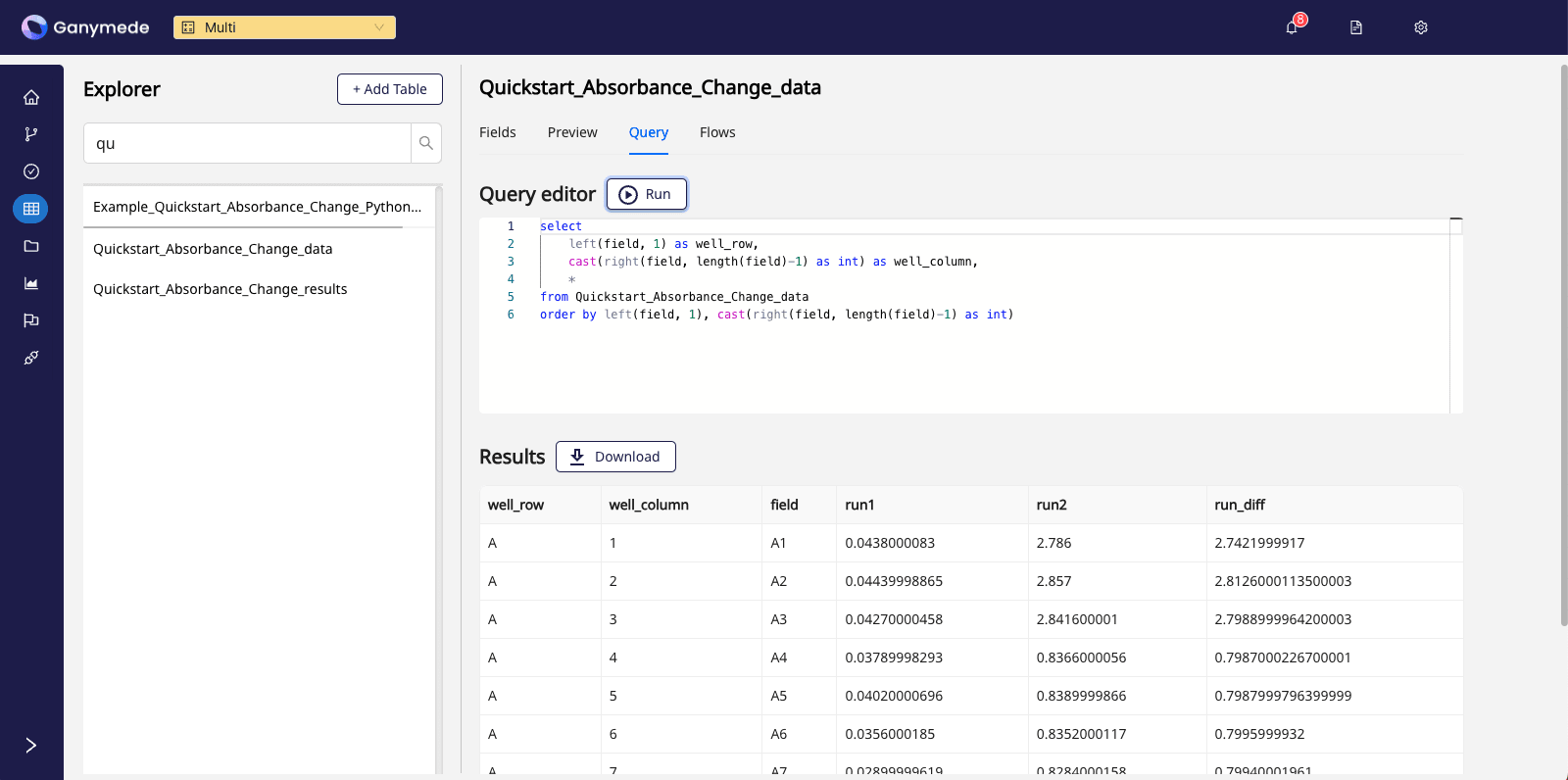
For example, clicking on the Query tab and running the query below:
select
    left(field, 1) as well_row,
    cast(right(field, length(field)-1) as int) as well_column,
    *
from Quickstart_Absorbance_Change_data where field not in ('Cycle Nr.', 'Time [s]', 'Temp. [°C]')
order by left(field, 1), cast(right(field, length(field)-1) as int)
yields a view of the plate reader results submitted:
If you run into any challenges with the Quickstart, please visit the Troubleshooting Flows page or contact Ganymede Support.
Exploring additional features
Schema validation
You may have noticed a Pandera snippet in the User-Defined Function cell of the Python node. This is a schema validation library that can be used to validate the structure of the data returned by the User-Defined Function. An example for validating that output only contains plate reader data with measurements (i.e. - no metadata) is shown below:
import pandas as pd
from ganymede_sdk.io import NodeReturn
from typing import Union, Dict, List

from pandera import Column, DataFrameSchema, Check
import re

schema = DataFrameSchema(
    {
        "field": Column(str,
                        Check.str_matches(r'\w\d\d?'),
                        required=True,
                        nullable=False
                       ),
        "run1": Column(float, required=True, nullable=False),
        "run2": Column(float, required=True, nullable=False)
    }
)

def execute(
    df_sql_result: Union[pd.DataFrame, List[pd.DataFrame]], ganymede_context=None
) -> Union[pd.DataFrame, Dict[str, pd.DataFrame]]:

    # remove fields that do not contain well measurements
    df_out = df_sql_result[~df_sql_result['field'].isin(['Cycle Nr.', 'Time [s]', 'Temp. [°C]'])].copy()

    # calculate absorbance difference
    df_out['run_diff'] = df_out['run2'] - df_out['run1']

    schema.validate(df_out)

    return NodeReturn(
        tables_to_upload={'Quickstart_Absorbance_Change_data': df_out},
    )